Ternary Plots in R with Plotly

Introduction

Ternary Plots enable us to visualize 3 parameters simultaneously on a plane. The proportion of the 3 variables must sum up to a constant.

Data

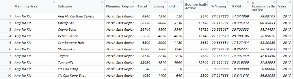
In a previous post we created bubble plots based on the proportion of young and economically active in Singapore’s subzones. However we were unable to plot the proportion of the old in the same graph. This set of data is ideal for a ternary plot. We will use the Singapore population data available from Singstat. Population data in the various residential subzones, planning areas and planning regions are available from 2002 to 2017. Singstat breaks down the population by 5 year cohorts; 0-4 years old, 5-9 years old, and so forth. For our analysis we will group the population into young (0-24 years old), economically active (25-64 years old) and old (65 years and above). Here is the header of our table

Ternary Plot

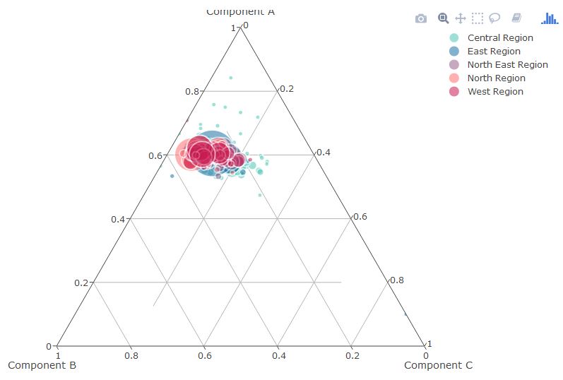
Plotly is plots ternary diagrams when the argument type is set to "scatterternary". Instead of specifyign the x and y axes, we specify a, b and c, set to % Young, % Economically Active and %Old respectively. Like in the bubble plot, the size of the bubble represents the total population in the subzone while the subzones are colored by Planning Region.

library(ggplot2)
library(plotly)
# we filter out data with zero %
tern %>%filter(`% Young`!=0 & `% Old`!=0 & `% Economically Active`!=0 & !is.na(`Planning Region`))%>%
        filter(Year>=2010)
tern2017<-tern %>% filter(Year=='2017')

# we create the ternary plot using plotly
p1<- plot_ly(
  tern2017, a = ~`% Economically Active`, b = ~`% Young`, c = ~`% Old`,
  color = ~`Planning Region`, type = "scatterternary", colors=~colors,
  size = ~Total,
  text = ~paste('Young:',sep='', round(`% Young`,1),'%',
                '<br>Economically Active:',
                round(`% Economically Active`,1),'%', '<br>Old:',
                round(`% Old`,1),'%','<br>Subzone:', Subzone, hoverinfo="text",
                      '<br>Planning Area:', `Planning Area`),
  marker = list(symbol = 'circle', opacity=0.55, sizemode="diameter", sizeref=1.5,
                      line = list(width = 2, color = '#FFFFFF')))

p1

We get the following ternary plot:

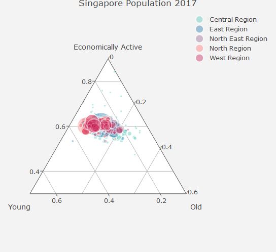
We can improve the plot by adding a title and limiting the range of the axes with the min parameter within the layout function.

# we create the ternary plot using plotly
p2 <- plot_ly(
  tern2017, a = ~`% Economically Active`, b = ~`% Young`, c = ~`% Old`,
  color = ~`Planning Region`, type = "scatterternary", colors=~colors,
  size = ~Total,
  text = ~paste('Young:',sep='', round(`% Young`,1),'%',
                '<br>Economically Active:',
                round(`% Economically Active`,1),'%', '<br>Old:',
                round(`% Old`,1),'%','<br>Subzone:', Subzone, hoverinfo="text",
                      '<br>Planning Area:', `Planning Area`),
  marker = list(symbol = 'circle', opacity=0.4, sizemode="diameter", sizeref=2,
                      line = list(width = 2, color = '#FFFFFF'))) %>%
  layout(
    title="Singapore Population 2017",
    ternary=list(aaxis=list(title="Economically Active",min=0.3),
    baxis = list(title="Young",min=0.1),
    caxis = list(title="Old")),
    paper_bgcolor = 'rgb(243, 243, 243)',
    plot_bgcolor = 'rgb(243, 243, 243)'
    )
p2

Improved plot:

Animation

Likewise, we animate using the frame parameter and edit the slider using the animation_opts function. Note that the bubbles only occupy a smaller portion of the ternary plot. For better visualization we limit the axes using the min parameter within the aaxis,baxis and caxis of the layout function. The Year is filtered after 2010 to limit the size of the table as plotly limits the upload size for free accounts.

# we create the ternary plot using plotly
p3 <- plot_ly(
  tern, a = ~`% Economically Active`, b = ~`% Young`, c = ~`% Old`,
  frame=~Year,
  color = ~`Planning Region`, type = "scatterternary", colors=~colors,
  size = ~Total,
  text = ~paste('Young:',sep='', round(`% Young`,1),'%',
                '<br>Economically Active:',
                round(`% Economically Active`,1),'%', '<br>Old:',
                round(`% Old`,1),'%','<br>Subzone:', Subzone, hoverinfo="text",
                      '<br>Planning Area:', `Planning Area`),
  marker = list(symbol = 'circle', opacity=0.4, sizemode="diameter", sizeref=2,
                      line = list(width = 2, color = '#FFFFFF'))) %>%
  layout(
    title="Singapore Population 2002-2017",
    ternary=list(aaxis=list(title="Economically Active",min=0.5),
    baxis = list(title="Young",min=0.2),
    caxis = list(title="Old")),
    paper_bgcolor = 'rgb(243, 243, 243)',
    plot_bgcolor = 'rgb(243, 243, 243)'
    ) %>%
  animation_slider(
    currentvalue = list(prefix = "YEAR ", font = list(color="red"))
  ) %>%
    animation_opts(
    2000, redraw = FALSE
  )
p3

We get the following ternary chart:

This gives us an overall picture of Singapore’s aging population compared to the bubble plot.