Imbalanced datasets with imbalanced-learn

Imbalanced Datasets with imbalanced-learn

1. Introduction

Machine learning classsification algorithms tend to produce unsatisfactory results when trying to classify unbalanced datasets. The number of observations in the class of interest is very low compared to the total number of observations. Examples of applications with such datasets are customer churn identification, financial fraud identification, identification of rare diseases, detecting defects in manufacturing, etc. Classifiers give poor results on such datasets as they favor the majority class, resulting in a high missclassification rate for the minority class of interest.

For example, when faced with a credit card fraud dataset where only 1% of transactions are fraudulent, a classification algorithm such as logistic regression would tend to predict that all transactions are legitimate, resulting in 99% accuracy. Needless to say, such an algorithm would be of little value. In real world cases, collecting more data might be an option and should be explored if possible.

To improve the prediction, our machine learning algorithms would require a roughly equal number of observations from each class. This new dataset can be constructed by resampling our observations. Imbalanced learn is a scikit-learn compatible package which implements various resampling methods to tackle imbalanced datasets. In this post we explore the usage of imbalanced-learn and the various resampling techniques that are implemented within the package.

2. Dataset

For our study we will use the Credit Card Fraud Detection dataset that has been made available by the ULB Machine Learning Group on Kaggle. The dataset contains almost 285k observations. The available features are Time, anonymous features V1 to V28(which are the results of PCA transformation) and Amount while the classification is given by class. Only 0.17% of the transactions are fraudulent.

import pandas as pd
df=pd.read_csv(r'C:\creditcard.csv')
df.head()

	Time	V1	V2	V3	V4	...	V26	V27	V28	Amount	Class
0	0.0	-1.359807	-0.072781	2.536347	1.378155	...	-0.189115	0.133558	-0.021053	149.62	0
1	0.0	1.191857	0.266151	0.166480	0.448154	...	0.125895	-0.008983	0.014724	2.69	0
2	1.0	-1.358354	-1.340163	1.773209	0.379780	...	-0.139097	-0.055353	-0.059752	378.66	0
3	1.0	-0.966272	-0.185226	1.792993	-0.863291	...	-0.221929	0.062723	0.061458	123.50	0
4	2.0	-1.158233	0.877737	1.548718	0.403034	...	0.502292	0.219422	0.215153	69.99	0

5 rows × 31 columns

3. Exploratory Data Analysis (EDA)

Although our goals is to see how the imbalanced-learn package work, we will still need to explore the data and correct for any issues as in any machine learning pipeline. In order to speed up the process, I referred to the kaggle kernals below:

• https://www.kaggle.com/joparga3/in-depth-skewed-data-classif-93-recall-acc-now/notebook
• https://www.kaggle.com/janiobachmann/credit-fraud-dealing-with-imbalanced-datasets

Of particular note, the Time and Amount are skewed:

import seaborn as sns
import matplotlib.pyplot as plt

fig, ax = plt.subplots(1, 2, figsize=(18,4))

amount_val = df['Amount'].values
time_val = df['Time'].values

sns.distplot(amount_val, ax=ax[0], color='r')
ax[0].set_title('Distribution of Transaction Amount', fontsize=14)
ax[0].set_xlim([min(amount_val), max(amount_val)])

sns.distplot(time_val, ax=ax[1], color='b')
ax[1].set_title('Distribution of Transaction Time', fontsize=14)
ax[1].set_xlim([min(time_val), max(time_val)])



plt.show()

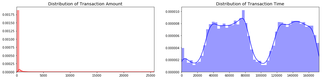
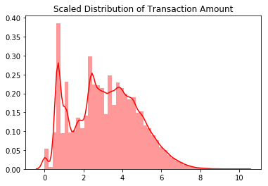
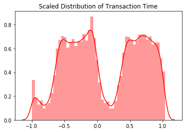
The transaction amount is heaviliy skewed towards small transactions and should be scaled. One option would be to use a log transformation on the data set. The transaction time seems to follow a night and day pattern with the number of transactions going down at night. As such I choose not to scale the time variable

import numpy as np
from sklearn.preprocessing import StandardScaler, RobustScaler

df['scaled_amount'] = np.log(df['Amount']+1)
rob_scaler = RobustScaler()
#df['scaled_amount'] = rob_scaler.fit_transform(df['Amount'].values.reshape(-1,1))
df['scaled_time'] = rob_scaler.fit_transform(df['Time'].values.reshape(-1,1))

#df.drop(['Amount'], axis=1, inplace=True)
df.drop(['Time','Amount'], axis=1, inplace=True)


scale_amount_val = df['scaled_amount'].values
sns.distplot(scale_amount_val, color='r').set_title("Scaled Distribution of Transaction Amount")
plt.show()

scale_time_val = df['scaled_time'].values
sns.distplot(scale_time_val, color='r').set_title("Scaled Distribution of Transaction Time")
plt.show()

C:\Users\david\AppData\Local\Continuum\Anaconda3\lib\site-packages\matplotlib\axes\_axes.py:6462: UserWarning: The 'normed' kwarg is deprecated, and has been replaced by the 'density' kwarg.
  warnings.warn("The 'normed' kwarg is deprecated, and has been "

4. Splitting the data into training and validation subsets

We split the data into the training and validation datasets cross-validation with a 70:30 ratio. This is a simple hold out method. Note that the training should be done on the rebalanced/resampled training dataset while the evaluation should be done one the original holdout validation dataset.

from sklearn.model_selection import train_test_split
y=df['Class']
x=df.drop(['Class'], axis=1)

x_train,x_test,y_train,y_test=train_test_split(x,y,test_size=0.3, stratify=y, random_state=0)

5. Training on an unbalanced dataset

Let us try to naively train bagging (decision tree) and random forest classifiers to our dataset. These 2 classifiers are chose for illustration purposes only and we will use sklearn default settings. The focus is not to find the best classifier and tune it, but to understand how to rebalanced skewed datasets. For our metric we will look at the confusion matrix of the test dataset.

from sklearn.ensemble import RandomForestClassifier
from sklearn.ensemble import BaggingClassifier
from sklearn.metrics import confusion_matrix
from sklearn.model_selection import cross_val_score


def fit_model(x_train,x_test,y_train,y_test):
    classifiers={"Random Forest":RandomForestClassifier(),
                 "Bagging-Decision Tree":BaggingClassifier(),}
    fig, ax = plt.subplots(1,2,figsize=(12,6))
    i=0

    for key, classifier in classifiers.items():
        classifier.fit(x_train, y_train)
        y_pred=classifier.predict(x_test)
        cm=confusion_matrix(y_test, y_pred)
        sns.heatmap(cm, ax=ax[i], annot=True,
                    cmap=plt.cm.Blues,
                   xticklabels=['No Fraud', 'Fraud'],
                   yticklabels=['No Fraud', 'Fraud']).set_title(key)

        i+=1
    plt.show()

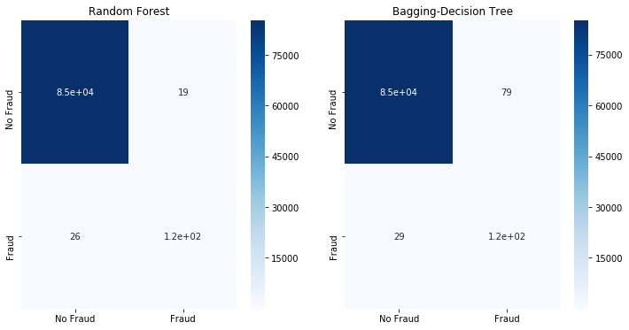
fit_model(x_train,x_test,y_train,y_test)

We observe that decision tree type classifiers are able to do a decent job to separate the Fraud and No Fraud classes although the classes are heavily imbalanced. This is usually not the case for imbalanced classes; the classifier typically classifies everything as belonging to the majority class.

5. Various techniques for resampling the training dataset

Here we explore the various options to rebalance the training dataset. The methods can either:

• Under-sample the majority class
• Over-sample the minority class.
• Combine over and under-sampling.
• Create ensemble balanced sets.

5.1 Undersampling the majority class

There are various algorithms implemented in imbalanced-learn that supports undersampling the majority class. They can be divided into generative and selective algorithms; generative algos try to summarize the majority class and then the samples are drawn from this generated data instead of the actual majority class observations. On the other hand, selective algorithms use various heuristics to select (or reject) samples to be drawn from the majority class. There are many undersampling algorithms and we will not run through all of them.

Undersampling with Random Under Sampler

The simplest selective under-sampler is the random under sampler RandomUnderSampler; we select the majority class randomly. Bootstrapping is possible by setting the parameter replacement to True.

from imblearn.under_sampling import RandomUnderSampler
rus = RandomUnderSampler(random_state=0)
x_rus, y_rus = rus.fit_sample(x_train, y_train)

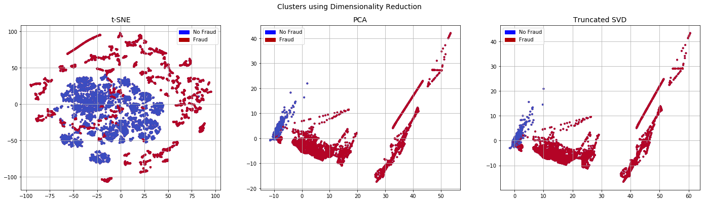
We also define the function plot_dim to display the data after t-SNE, PCA and Truncated SVD transformations.

from sklearn.manifold import TSNE
from sklearn.decomposition import PCA, TruncatedSVD
import time
import matplotlib.patches as mpatches


def plot_dim(x,y):
    # T-SNE Implementation
    t0 = time.time()
    X_reduced_tsne = TSNE(n_components=2, random_state=10).fit_transform(x)
    t1 = time.time()
    print("T-SNE took {:.2} s".format(t1 - t0))    

    # PCA Implementation
    t0 = time.time()
    X_reduced_pca = PCA(n_components=2, random_state=10).fit_transform(x)
    t1 = time.time()
    print("PCA took {:.2} s".format(t1 - t0))

    # TruncatedSVD
    t0 = time.time()
    X_reduced_svd = TruncatedSVD(n_components=2, algorithm='randomized', random_state=10).fit_transform(x)
    t1 = time.time()
    print("Truncated SVD took {:.2} s".format(t1 - t0))

    f, (ax1, ax2, ax3) = plt.subplots(1, 3, figsize=(24,6))
    # labels = ['No Fraud', 'Fraud']
    f.suptitle('Clusters using Dimensionality Reduction', fontsize=14)


    blue_patch = mpatches.Patch(color='#0A0AFF', label='No Fraud')
    red_patch = mpatches.Patch(color='#AF0000', label='Fraud')


    # t-SNE scatter plot
    ax1.scatter(X_reduced_tsne[:,0], X_reduced_tsne[:,1], s=4, c=(y == 0),
                cmap='coolwarm', label='No Fraud', linewidths=2)
    ax1.scatter(X_reduced_tsne[:,0], X_reduced_tsne[:,1], s=4, c=(y == 1),
                cmap='coolwarm', label='Fraud', linewidths=2)
    ax1.set_title('t-SNE', fontsize=14)

    ax1.grid(True)

    ax1.legend(handles=[blue_patch, red_patch])


    # PCA scatter plot
    ax2.scatter(X_reduced_pca[:,0], X_reduced_pca[:,1], s=4, c=(y == 0),
                cmap='coolwarm', label='No Fraud', linewidths=2)
    ax2.scatter(X_reduced_pca[:,0], X_reduced_pca[:,1], s=4, c=(y == 1),
                cmap='coolwarm', label='Fraud', linewidths=2)
    ax2.set_title('PCA', fontsize=14)

    ax2.grid(True)

    ax2.legend(handles=[blue_patch, red_patch])

    # TruncatedSVD scatter plot
    ax3.scatter(X_reduced_svd[:,0], X_reduced_svd[:,1], s=4, c=(y == 0),
                cmap='coolwarm', label='No Fraud', linewidths=2)
    ax3.scatter(X_reduced_svd[:,0], X_reduced_svd[:,1], s=4, c=(y == 1),
                cmap='coolwarm', label='Fraud', linewidths=2)
    ax3.set_title('Truncated SVD', fontsize=14)

    ax3.grid(True)

    ax3.legend(handles=[blue_patch, red_patch])

    plt.show()

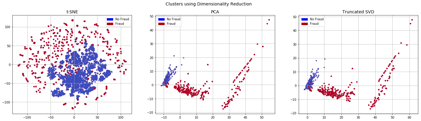
plot_dim(x_rus,y_rus)

T-SNE took 1.7e+01 s
PCA took 0.003 s
Truncated SVD took 0.002 s

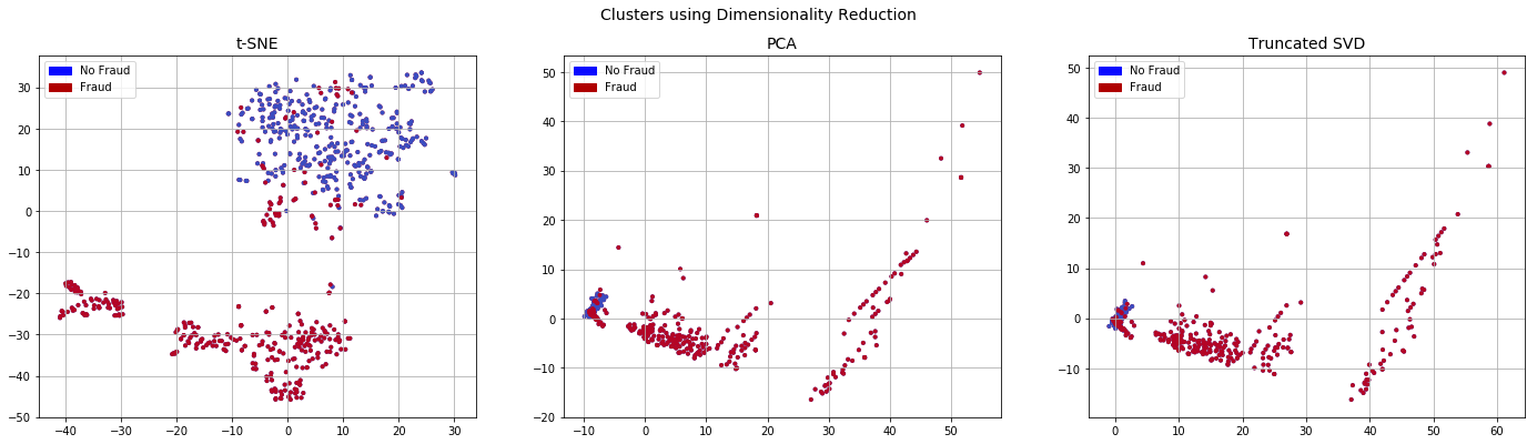
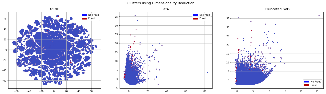
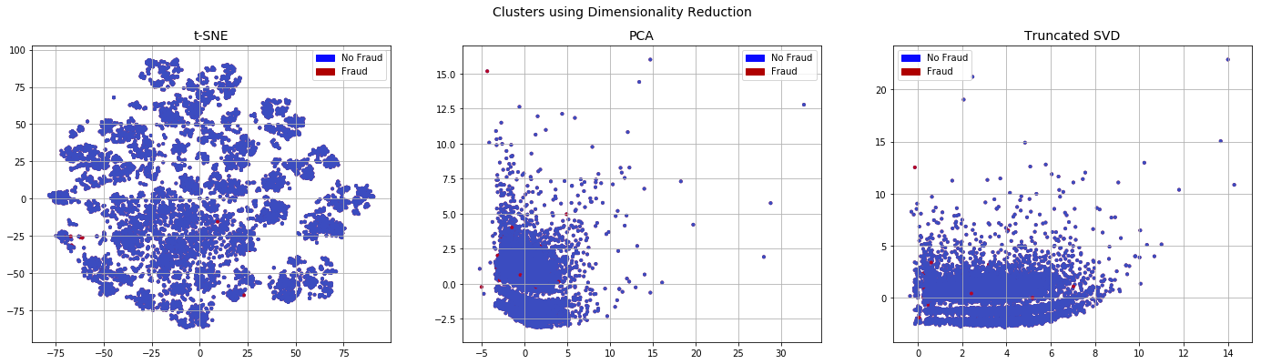
When we look at the data obtained from undersampling using dimensionality reduction, the No Fraud and Fraud classes appear separable. This is in contrast to the original imbalanced datasets where there are very few Fraud cases and they do not appear to be easily separable

x_train_plot,x_plot,y_train_plot,y_plot=train_test_split(x,y,test_size=0.2, stratify=y, random_state=0)
plot_dim(x_plot,y_plot)

T-SNE took 2.7e+03 s
PCA took 0.24 s
Truncated SVD took 0.17 s

Now that we have the used Random Undersampling to replaced the classes, we use a classifier to see how the model would perform when trained on a rebalanced dataset.

fit_model(x_rus,x_test,y_rus,y_test)

Although more of the Fraud classes are detected, this comes at an elevated False Positive rate - we will label more than 2k No Fraud cases as Fraud. When undersampling the majority or No Fraud class. It appears that we have oversimplified it, causing classification errors.

Under Sampling with Tomek Links

The classifier detects Tomek’s Links : this link exists if 2 samples from different classes are the nearest neighbours of each other. The sample from the majority class is then removed from the dataset.

from imblearn.under_sampling import TomekLinks
tomekl = TomekLinks(random_state=0,n_jobs=3)
x_tomekl, y_tomekl = tomekl.fit_sample(x_train, y_train)

from sklearn.utils import resample
x_tomekl_plot,y_tomekl_plot=resample(x_tomekl,y_tomekl,n_samples=10000,random_state=0)
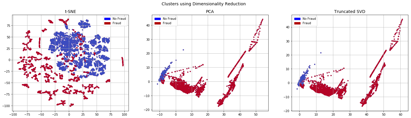
plot_dim(x_tomekl_plot,y_tomekl_plot)

T-SNE took 3.6e+02 s
PCA took 0.028 s
Truncated SVD took 0.025 s

Even after running TomekLinkwe observe that the dataset is similar to the initial imbalanced dataset. Thus it is unsurprising to get similar classification results as shown below.

fit_model(x_tomekl,x_test,y_tomekl,y_test)

5.2 Oversample the minority class

Instead of reducing the majority class. We can choose to oversample the minority class instead to rebalance the dataset.

Random Over Sampling

In Random Oversampling, the we favor the minority class when sampling to rebalance the dataset.

from imblearn.over_sampling import RandomOverSampler
ros = RandomOverSampler(ratio='minority',random_state=0)
x_ros, y_ros = ros.fit_sample(x_train, y_train)

x_ros_plot,y_ros_plot=resample(x_ros,y_ros,n_samples=10000,random_state=0)
plot_dim(x_ros_plot,y_ros_plot)

T-SNE took 3.2e+02 s
PCA took 0.038 s
Truncated SVD took 0.025 s

Random over sampling gives us a more separable dataset. We obtained slightly better results for the Random Forest classifier.

fit_model(x_ros,x_test,y_ros,y_test)

SMOTE

SMOTE or Synthetic Minority Over-Sampling Technique creates additional samples of the minority class. The parameter k_neighbors determines the number of neighbours of the minority class to consider when creating synthetic data. The new datapoint is created somewhere between these k neighbours. Refer to the original article for more information

from imblearn.over_sampling import SMOTE
sm = SMOTE(random_state=0)
x_smote, y_smote = sm.fit_sample(x_train, y_train)

x_smote_plot,y_smote_plot=resample(x_smote,y_smote,n_samples=10000,random_state=0)
plot_dim(x_smote_plot,y_smote_plot)

T-SNE took 3.3e+02 s
PCA took 0.033 s
Truncated SVD took 0.023 s

We observe that the resulting dataset is less separable compared to the random over sampled dataset, especially after running t-SNE.

fit_model(x_smote,x_test,y_smote,y_test)

5.3 Combine oversampling and undersampling

It is also possible to combine both over sampling and undersampling to rebalance the datasets.

SMOTE ENN

SMOTE ENN combines SMOTE (over sampling) and ENN or Edited Nearest Neighbours (Under Sampling)

from imblearn.combine import SMOTEENN
enn = SMOTEENN(random_state=0)
x_enn, y_enn = enn.fit_sample(x_train, y_train)

x_enn_plot,y_enn_plot=resample(x_enn,y_enn,n_samples=10000,random_state=0)
plot_dim(x_enn_plot,y_enn_plot)

T-SNE took 3.3e+02 s
PCA took 0.034 s
Truncated SVD took 0.023 s

fit_model(x_enn,x_test,y_enn,y_test)

SMOTE TOMEK

SMOTE TOMEK combines SMOTE (over sampling) and Tomek links (Under Sampling)

from imblearn.combine import SMOTETomek
stomek = SMOTETomek (random_state=0)
x_stomek, y_stomek = stomek.fit_sample(x_train, y_train)

x_stomek_plot,y_stomek_plot=resample(x_stomek,y_stomek,n_samples=10000,random_state=0)
plot_dim(x_stomek_plot,y_stomek_plot)

T-SNE took 3.2e+02 s
PCA took 0.036 s
Truncated SVD took 0.024 s

fit_model(x_stomek,x_test,y_stomek,y_test)

Neither SMOTE ENN nor SMOTE Tomek are able to improve the classification results.

5.4 Ensemble Balancing

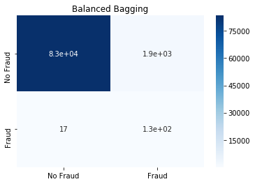
Balanced Bagging Classifier

This is essentially a bagging classifier with additional balancing. We try it out with the default Decision Tree and Support Vector Machine classifier.

from imblearn.ensemble import BalancedBaggingClassifier
bb=BalancedBaggingClassifier(random_state=0, n_jobs=3)
bb.fit(x_train, y_train)

y_pred=bb.predict(x_test)
cm=confusion_matrix(y_test, y_pred)
sns.heatmap(cm, annot=True,
                    cmap=plt.cm.Blues,
                   xticklabels=['No Fraud', 'Fraud'],
                   yticklabels=['No Fraud', 'Fraud']).set_title('Balanced Bagging')

from sklearn.svm import SVC
bbsvm=BalancedBaggingClassifier(base_estimator=SVC(),n_estimators=50,random_state=0, n_jobs=3)
bbsvm.fit(x_train, y_train)

y_pred=bbsvm.predict(x_test)
cm=confusion_matrix(y_test, y_pred)
sns.heatmap(cm, annot=True,
                    cmap=plt.cm.Blues,
                   xticklabels=['No Fraud', 'Fraud'],
                   yticklabels=['No Fraud', 'Fraud']).set_title('Balanced Bagging - SVM')

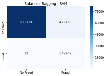
The Balanced Bagging SVM classifier is able to detect the highest amount of Fraud, at the cost of high false positives for No Fraud

Conclusion

We have run through the various options in imbalanced-learn to rebalance and imbalanced dataset. However the original imbalanced dataset can already be classified relatively well. As such it is more difficult to illustrate the full benefits of rebalancing the dataset.

This post was written as a Jupyter Notebook. Click here to view it.