Faceted Population Pyramids

Introduction

Population Pyramids are a specific type of bar chart that allows us to easily visualize the age and sex distribution of the population. A population pyramid allows us to clearly distinguish between countries or regions with high fertility (wide pyramid base) and low fertility (narrow pyramid base).

Data

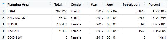
We will use the Singapore population data available from Singstat. Population data in the various residential subzones, planning areas and planning regions are available from 2002 to 2017. Singstat breaks down the population by gender into 5 year cohorts; 0-4 years old, 5-9 years old, and so forth, which is exactly what we need to build a population pyramid.

This excel dataset, tablea12-2000-2017.xls is poorly formatted and the data has to be processed to extract the data of interest. Multiple tables are placed in a same excel sheet with many blanks in the data. The data format also varies between excel sheets as the geographical subzones change in 2011.

We read in the table with readxl and we need to specify the exact line where the tables start.

library(tidyverse)

read_male <- function(filename) {
    sheets <- readxl::excel_sheets(filename)[1:7]
    x <-    lapply(sheets, function(X) readxl::read_excel(filename, sheet = X, skip=393)
                   %>% slice(2:380) %>% fill(`Planning Area`) %>% mutate_at(.cols=vars(3:21),.funs=as.integer)
                   %>% filter(Subzone=="Total")
                   %>% replace_na(replace=list(`Total`=0,`0 - 4`= 0,`5 - 9`= 0,`10 - 14`=0,`15 - 19`=0,
                                               `20 - 24`=0,`25 - 29`=0, `30 - 34`=0, `35 - 39`=0,
                                               `40 - 44` =0, `45 - 49` =0, `50 - 54`=0, `55 - 59`=0,
                                               `60 - 64` = 0, `65 - 69`=0, `70 - 74`=0, `75 - 79`=0,
                                               `80 - 84`=0, `85 & Over`=0))
                   %>% rename(`05 - 09`=`5 - 9`,`00 - 04`=`0 - 4`)
                   %>% mutate(Gender="Male",
                              `Planning Area`=toupper(`Planning Area`))
                     )


    names(x) <- sheets
    x
}

read_female <- function(filename) {
    sheets <- readxl::excel_sheets(filename)[1:7]
    x <-    lapply(sheets, function(X) readxl::read_excel(filename, sheet = X, skip=784)
                   %>% slice(2:380) %>% fill(`Planning Area`) %>% mutate_at(.cols=vars(3:21),.funs=as.integer)
                   %>% filter(Subzone=="Total")
                   %>% replace_na(replace=list(`Total`=0,`0 - 4`= 0,`5 - 9`= 0,`10 - 14`=0,`15 - 19`=0,
                                               `20 - 24`=0,`25 - 29`=0, `30 - 34`=0, `35 - 39`=0,
                                               `40 - 44` =0, `45 - 49` =0, `50 - 54`=0, `55 - 59`=0,
                                               `60 - 64` = 0, `65 - 69`=0, `70 - 74`=0, `75 - 79`=0,
                                               `80 - 84`=0, `85 & Over`=0))
                   %>% rename(`05 - 09`=`5 - 9`,`00 - 04`=`0 - 4`)
                   %>% mutate(Gender="Female",`Planning Area`=toupper(`Planning Area`))
                     )


    names(x) <- sheets
    x
}

male_total <- read_male("tablea12-2000-2017.xls")
female_total <- read_female("tablea12-2000-2017.xls")

Not the neatest way but we add the Year information into the dataset :

male_0<-male_total[[1]] %>% mutate(Year=2017)
male_1<-male_total[[2]] %>% mutate(Year=2016)
male_2<-male_total[[3]] %>% mutate(Year=2015)
male_3<-male_total[[4]] %>% mutate(Year=2014)
male_4<-male_total[[5]] %>% mutate(Year=2013)
male_5<-male_total[[6]] %>% mutate(Year=2012)
male_6<-male_total[[7]] %>% mutate(Year=2011)

female_0<-female_total[[1]] %>% mutate(Year=2017)
female_1<-female_total[[2]] %>% mutate(Year=2016)
female_2<-female_total[[3]] %>% mutate(Year=2015)
female_3<-female_total[[4]] %>% mutate(Year=2014)
female_4<-female_total[[5]] %>% mutate(Year=2013)
female_5<-female_total[[6]] %>% mutate(Year=2012)
female_6<-female_total[[7]] %>% mutate(Year=2011)

The male population is assigned negative values so that it appears on the left. Since there are multiple planning areas we display the percentage instead of the absolute population value.

male_final<-bind_rows(male_0,male_1,male_2,male_3,male_4,male_5,male_6) %>%
  select(-Subzone) %>%
  gather(key=Age,value = Population,`00 - 04`:`85 & Over`) %>%
  mutate(Population=-Population)%>%
  group_by(Year,`Planning Area`) %>%
  mutate(Percent=-Population/sum(Population)*100)

female_final<-bind_rows(female_0,female_1,female_2,female_3,female_4,
                     female_5,female_6) %>%
  select(-Subzone) %>%
  gather(key=Age,value = Population,`00 - 04`:`85 & Over`)%>%
  group_by(Year,`Planning Area`) %>%
  mutate(Percent=Population/sum(Population)*100)

pop_final<-bind_rows(female_final,male_final)

Finally we get the pop_final dataframe:

Population Pyramid with ggplot2

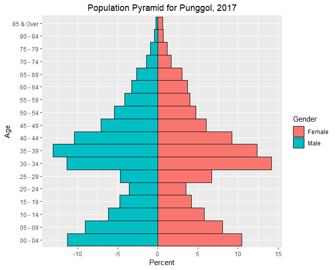
To create a pyramid with ggplot we filter the dataset for 2017 and Planning Area == PUNGGOL.

pyramid<-pop_final %>%
  filter(`Planning Area` =='PUNGGOL', Year==2017)

Since we have already assigned negative values for males. We just have to assign the correct aesthetics within aes. To remove spacing between bars, we set the parameter width=1 within the geom_bar function.

library(ggplot2)
ggplot(pyramid, aes(x=Age,fill=Gender,y=Percent))+
  geom_bar(stat="identity",width=1,color="black")+
  ggtitle("Population Pyramid for Punggol, 2017")+
  theme(plot.title = element_text(hjust = 0.5))+
  coord_flip()

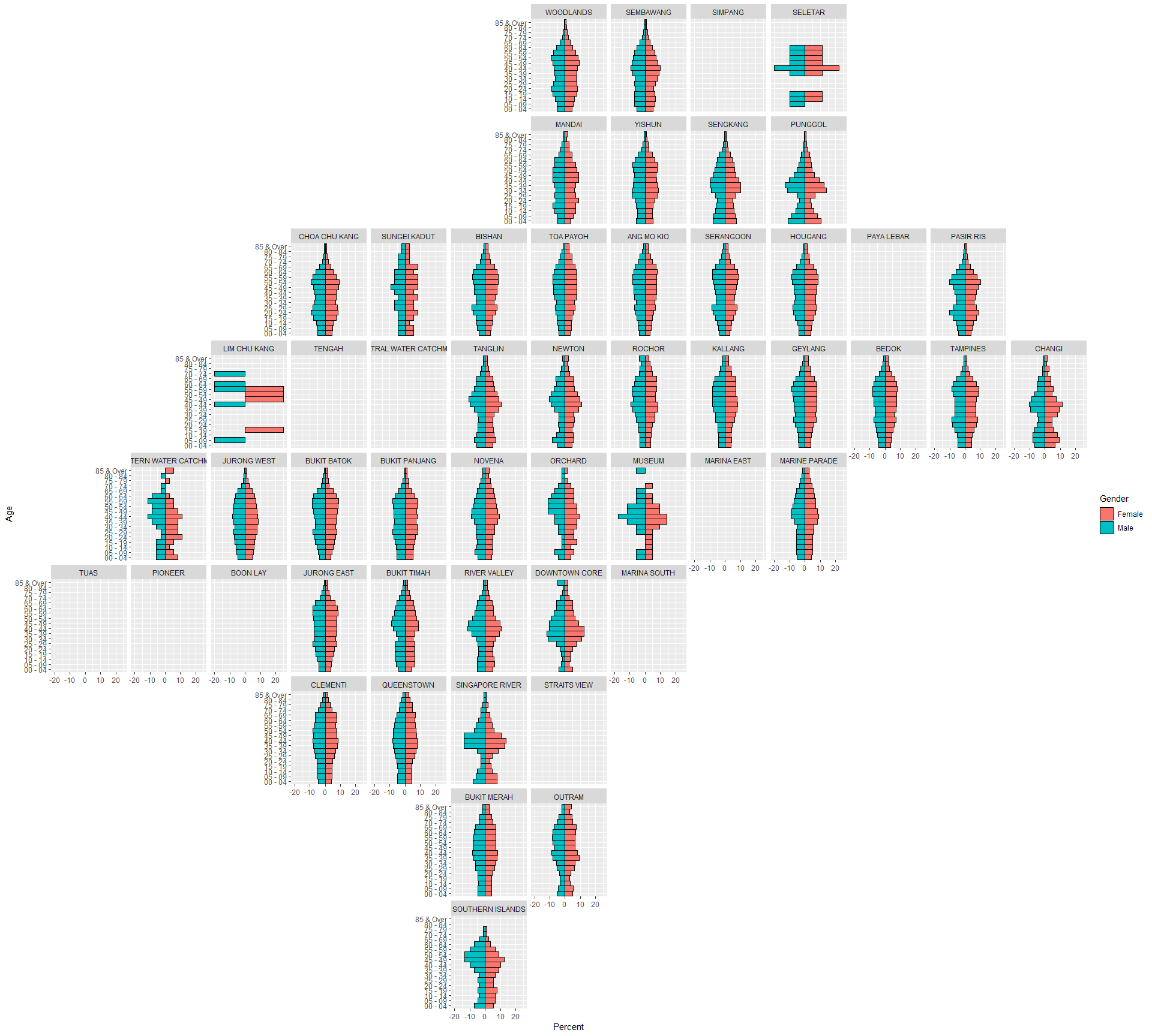
Geofacet

geofacet is an R package that extends ggplot2's faceting capabilities. Instead of creating uniform facets, the facets are mapped onto a grid representing the geographical location of the various regions or states of a country. The parameter grid of the function facet_geo allows us to select the country grid. Unfortunately, Singapore is not on the list of possible grids. As such a user grid has to be created. We use the proposed Singapore grid in this github issue

library(geofacet)
geo<-pop_final %>%
  filter(Year==2017)%>% rename(name=`Planning Area`)

sggrid<-read.csv("mygrid.csv")
m<-ggplot(geo, aes(x=Age,fill=Gender,y=Percent))+
  geom_bar(stat="identity",width=1,color="black")+
  coord_flip()+
  facet_geo(vars(name),grid = sggrid)
m