Isochrone Maps with R and OpenTripPlanner

Introduction

Isochrone Maps depict areas of equal travel time from a certain point of departure. They are particularly useful for urban transport and hydrology. For example we can easily visualize how long it would take to travel to a point of interest, like to airports or central business districts. If we are interested in buying or renting property then it would be helpful to visualize how well of poorly connected the property is. Typically we would display multiple time intervals to depict successively larger areas that can be reached as the travel time increases.

An example of such a visualization for Singapore’s public transport is Shan Yang’s isochrone which can display isochrones for various addresses that the user can key in the search bar. Previously, mapzen provided an API for isochrones but unfortunately they went out of business. Fret not, it can still be built from scratch.

GTFS

To create an public transport isochrone we would need information about the various modes of public transport, the schedule, location of the stops, etc. General Transit Feed Specification or GTFS is a standardized format for public transportation schedules created by Google. GTFS is typically used as input to plan multi stop journeys on public transport. The 6 compulsory tables are :

1. agency - transit agency
2. routes - distinct routes. In Singapore this could be a bus number, or an MRT line , e.g. Downtown Line
3. trips
4. stop_times
5. stops - geographic locations of the stops
6. calendar - this defines the service pattern

Singapore’s transport agencies to not provide data directly in GTFS format but it is possible to scrape the various websites to establish this information. Fortunately Shan Yang has generously shared the data in his singapore-gtfs repository. The data is for weekdays only and frequencies are averaged out. This is perfectly fine as we want to generate isochrones and not schedule trips.

OpenTripPlanner

OpenTripPlanner or OTP is an open source trip planner which requires GTFS data (in a .zip file) and Open Street Map data of the geographical area of interest, typically in PBF format as input. It is available as a runnable JAR file. Marcus Young has a very good tutorial on how to get the OTP server up and running, usually on http://localhost:8080. While OTP will allow us to plan trips, it can also calculate isochrones based on the GTFS data available to it.

Queries can be sent to the server via R or python while the server is up and running. the function get_geojson below will request the isochrone for a certain latitude and longitude. We also need to give OTP certain parameters for the query.

• cutoffSec is the travel time that we are interested in (multiple cutoffs can be requested)
• mode is the mode of transport
• maxWalkDistance gives the maximum that distance that we expect the user to walk.
• walkReluctance is a multiplier for how bad walking is, compared to being in transit

library(httr)
get_geojson<-function(lat,lng,filename){

current <- GET(
  "http://localhost:8080/otp/routers/current/isochrone",
  query = list(
    fromPlace = paste(lat,lng,sep = ","), # latlong of place
    mode = "WALK,TRANSIT", # modes we want the route planner to use
    date = "07-10-2018",
    time= "08:00am",
    maxWalkDistance = 1600, # in metres
    walkReluctance = 5,
    minTransferTime = 60, # in secs
    cutoffSec = 900,
    cutoffSec = 1800,
    cutoffSec = 2700,
    cutoffSec = 3600
  )
)

current <- content(current, as = "text", encoding = "UTF-8")
write(current, file = paste("C:/geojson/",filename,".geojson"))
}

In return we get a .geojson which we can then display.

Isochrone with R Leaflet

Now that we have a geojson file, we can overlay it onto the map of Singapore with leaflet. For example we get the isochrone for Changi Airport Terminal 1. The latitude and longitude can be found using the OneMap API (refer to this post

get_geojson(1.36173580440684,
  103.990348825503,
  "Changi-Terminal-1")

We can then display the isochrone using leaflet. The .geojson file can be read in as an sp object using the geojsonio package function geojson_read.

library(tidyverse)
library(leaflet)

iso <- geojsonio::geojson_read("C:/Users/david/geojson/SMU.geojson",
  what = "sp")

pal=c('cyan','gold','tomato','red')

m<-leaflet(iso) %>%
    setView(lng = 103.8198, lat = 1.3521, zoom = 11) %>%
  addProviderTiles(providers$CartoDB.DarkMatter,
                   options = providerTileOptions(opacity = 0.8))%>%  
  addPolygons(stroke = TRUE, weight=0.5,
              smoothFactor = 0.3, color="black",
              fillOpacity = 0.1,fillColor =pal ) %>%
  addLegend(position="bottomleft",colors=rev(c("lightskyblue","greenyellow","gold","tomato")),
            labels=rev(c("60 min","45 min",
                     "30 min","15 min")),
            opacity = 0.6,
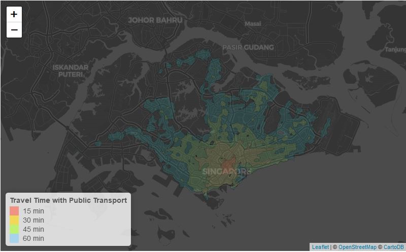
            title="Travel Time with Public Transport")

m

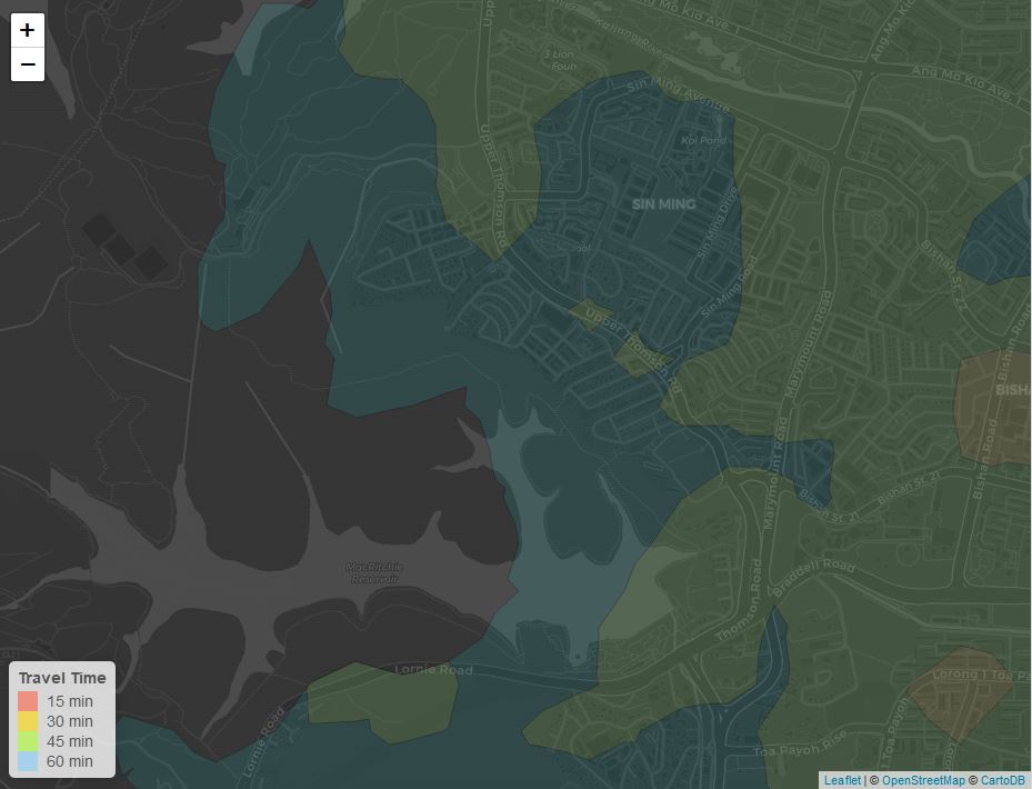
In the interactive leaflet output below we can see Changi Airport is mainly connected via the East-West line and it would take a traveler an hour to reach the CBD.

We can also take a look at how well connected the major universities (NUS, NTU and SMU ) in Singapore are:

NUS

NTU

SMU

SMU being in the CBD is very well connected whereas poor NTU students are really cut off, being located in the West of Singapore without an MRT station.

The isochrone allows us to visualize how connected a place is via public transport and depends on the parameters sent to OTP. As we have the geojson file we can perform calculations such as determining the area covered, overlaps, etc. Since we built the isochrone from the GTFS, we can see the impact of adding new transport routes or the impact of disruptions when certain routes are cut off by modifying the transit rules. We can also set up an OpenTripPlanner server and allow the user to query locations with different trip parameters.

Note that the settings might still have some errors as barriers to walking are not taken into account. For example, it does not recognize bodies of water, and actually shows that a commuter can walk on the MacRitchie reservoir!