Bubble Plots to Visualize Singapore Private Property

Introduction

Having seen choropleths and bubble plots, we now examine how to display bubble plots on maps. In particular, we would like to display the location of private properties in Singapore. The Markers vignette for R leaflet gives a quick introduction on how to display markers on maps.

Data

Our dataset, Private2017.csv contains summarized property transaction data. To correctly display property in such, we will need accurate geolocation data. Fortunately OneMap provides excellent geolocation data, which can accessed via their API.

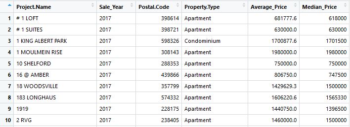
We use the postcode from our data to systematically retrieve the longitude and latitude of the various private properties that were sold in 2017. As we have the individual postcodes, we are able to distinguish between blocks within a project. OneMap limits us to 250 API calls per minute.

import time
import requests
import simplejson as json
import pandas as pd

df_postcode=pd.read_csv("D:/private2017.csv",dtype=str)

for i in range(len(df_postcode)):
    if len(str(df_postcode['Postal.Code'][i]))==5:
        df_postcode['Postal.Code'][i]='0'+df_postcode['Postal.Code'][i]
df_postcode['OnemapLongitude'] = pd.Series(0, index=df_postcode.index)
df_postcode['OnemapLatitude'] = pd.Series(0, index=df_postcode.index)       

start=time.time()
for i in range(len(df_postcode)):
    req=requests.get('https://developers.onemap.sg/commonapi/search?searchVal='+df_postcode['Postal.Code'][i]+'&returnGeom=Y&getAddrDetails=Y&pageNum=1')
    jdata = json.loads(req.text)
    if jdata['found']>=1:
        df_postcode['OnemapLongitude'][i]=jdata['results'][0]['LONGITUDE']
        df_postcode['OnemapLatitude'][i]=jdata['results'][0]['LATITUDE']
    else:
        df_postcode['OnemapLongitude'][i]=float('nan')
        df_postcode['OnemapLatitude'][i]=float('nan')
df_postcode.to_csv("D:/private2017-longlat.csv")
print('Time Taken:',time.time()-start)

Similarly, we starting from a list of MRT station names MRT.csv in our data folder, we can find the position of the MRT stations in Singapore. Note that OneMap can return the location of the MRT exits or just a central location. For our application we would like to determine the distance to the nearest MRT exit. As such we will request the location of all exits

mrt="D:/MRT.csv"
df_mrt_names=pd.read_csv(mrt,header=None)

df_mrt=pd.DataFrame(columns=['MRT','long','lat'])

for i in range(len(df_mrt_names)):
    time.sleep(0.3)
    req=requests.get('https://developers.onemap.sg/commonapi/search?searchVal='+df_mrt_names[0][i]+'&returnGeom=Y&getAddrDetails=Y&pageNum=1')
    jdata = json.loads(req.text)
    if jdata['found']>=1:
        for j in range(min(jdata['found'],10)):
            if 'MRT STATION EXIT' in jdata['results'][j]['ADDRESS']:
                df_new=pd.DataFrame(np.random.randint(low=0, high=10, size=(1, 3)),columns=['MRT','long','lat'])
                df_new['MRT'][0]=jdata['results'][j]['ADDRESS']
                df_new['long'][0]=jdata['results'][j]['LONGITUDE']
                df_new['lat'][0]=jdata['results'][j]['LATITUDE']
                df_mrt=df_mrt.append(df_new)

Distance to nearest MRT

The distance between 2 points can be accurately calculated using Vincenty’s formula. It is possible to implement our own calculation using the math library in python. Another option is to install the vincenty library and call the vincenty function for our calculations (the function returns the distance in meters). In R, the geosphere package has the vincenty formulae implemented as well and returns a distance matrix. However the downside is that it is single threaded and consumes a large amount of memory. To calculate the nearest MRT alone we have around 6400 properties and 500 MRT station exits, requiring in 3.2M calculations.

from vincenty import vincenty
import pandas as pd
from multiprocessing import Pool
import time
from itertools import product

def postcode_vincenty(mrt,prop):
    dist=vincenty(mrt[1:],prop[1:])*1000
    return((prop[0],)+(mrt[0],)+(dist,))    

if __name__ == '__main__':
    ## Read Data
    mrt=pd.read_csv('MRT_lat_long.csv')
    prop=pd.read_csv('private2017-longlat.csv')
    ## Convert to List of tuples
    mrt=[(mrt['MRT'][i],mrt['lat'][i],mrt['long'][i]) for i in range(len(mrt))]
    prop=[(prop['Postal.Code'][i],prop['OnemapLatitude'][i],prop['OnemapLongitude'][i]) for i in range(len(prop))]

    p = Pool(4)  
    start=time.time()
    results=p.starmap(postcode_vincenty,product(mrt,prop))
    p.terminate()
    p.join()
    data=pd.DataFrame(results,columns=['Postcode','MRT Exit','Distance(m)'])
    data=data.sort_values("Distance(m)").groupby("Postcode", as_index=False).first()
    print('Time Taken:',time.time()-start)
    data.to_csv('vincenty.csv')

We can also calculate the nearest private properties with slight modification to the codes, and this will require almost 41M calculations.

Leaflet and Bubble Plots

Previously we used the addPolygons function in leaflet to produce choropleths. To add bubbles in specific locations, we use the addCircles function. The parameters lng and lat refer to the longitude and latitude. The radius determines the size of the bubble, which we set to be proportional to the square root of the average price. We can also display a pop up when the user’s mouse hovers over the bubble. In our case we display the project name, average price, nearest MRT and distance to MRT. A bit of html is required to separate the attributes as \n does not work here. We use the htmltools package to convert to HTML. Refer to this post on stackoverflow for more information.

library(tidyverse)
library(leaflet)
library(htmltools)

# Read In data
property<-read.csv("D:/private2017-longlat.csv")
mrt<-read.csv("C:/Users/david/Desktop/vincenty.csv")


# Join MRT data and property data
property<-merge(property,mrt,by.x="Postal.Code", by.y = "Postcode")


# Define color palette
pal <- colorFactor(c('#4AC6B7', '#1972A4', '#965F8A',
 '#FF7070', '#C61951',"gold"), domain = c("Detached House",
 "Apartment","Condominium","Executive Condominium",
 "Semi-Detached House","Terrace House"))


# Create html for new lines in label
labs <- lapply(seq(nrow(property)), function(i) {
  paste0( '<b>Project Name: </b>', property[i, "Project.Name"], '</br>',
          '<b>Average Price($): </b>',property[i, "Average_Price"],'</br>',
          '<b>Nearest MRT: </b>',property[i, "MRT.Exit"],'</br>',
          '<b>Distance to MRT (m): </b>',property[i, "Distance.m."],'</br>')
})




m <- leaflet(property) %>%
  setView(lng = 103.8198, lat = 1.3521, zoom = 12) %>%
  setMaxBounds( lng1 = 103.600250,
                lat1 = 1.202674,
                lng2 = 104.027344,
                lat2 = 1.484121 )%>%
  addTiles(options=tileOptions(opacity=0.6)) %>%  
  addCircles(lng=~OnemapLongitude, lat=~OnemapLatitude,
           radius=~sqrt(Average_Price/500),
           color=~pal(Property.Type),
           weight=2,
           label=lapply(labs, HTML),
           stroke=TRUE,opacity=0.8,fillOpacity=0.5,
           #clusterOptions=markerClusterOptions(),
           layerId = ~Project.Name) %>%
  addLegend("topright", pal = pal,
          values = ~Property.Type,
          title = "Property Type",
          opacity = 1)

m