Time Series Forecasting with Prophet
Introduction
Time series forecasting is used in multiple business domains, such as pricing, capacity planning, inventory management, etc. Forecasting with techniques such as ARIMA requires the user to correctly determine and validate the model parameters . This is a multistep process that requires the user to interpret the Autocorrelation Function (ACF) and Partial Autocorrelation (PACF) plots correctly. Using the wrong model can easily lead to erroneous results.
Prophet is an open source time series forecasting library made available by Facebook’s Core Data Science team. It is available both in Python and R, and it’s syntax follow’s Scikit-learn’s train and predict model.
Prophet is built for business cases typically encounted at Facebook, but which are also encountered in other businesses:
- Hourly, Daily or Weekly data with sufficient historical data
- Multiple Seasonality patterns related to human behaviour (day of week, seasons)
- Important holidays that are irregularly spaced (Thanksgiving, Chinese New Year, etc.)
- Reasonable amount of missing data
- Historical trend changes
- Non linear growth trends with saturation (capacity limit, etc.)
The goal of Prophet is to product high quality forecasts for decision making out of the box without requiring the user to have expert time series forecasting knowledge. The user can intuitively intervene during the model building process by introducing known parameters such as trend changepoints due to product introduction or trend saturation values due to capacity.
Stan
Prophet uses Stan as its optimization engine to fit its model and calculate uncertainty intervals. Stan is installed along with the R or Python libraries when Prophet is installed. Stan performs Maximum a Priori (MAP) optimization by default but if sampling can be requested.
Data
According to Facebook, Prophet is able to give accurate forecasting results with it’s default settings, little or no tuning required. Let’s test out Prophet using two different datasets:
We’ll use the python library as there not many time series forecasting libraries in this language whereas R has popular packages such as forecast, tseries, etc.
We’ll load the tanker data into the dataframe tanker and the flight passenger data into the dataframe air.
import pandas as pd
from fbprophet import Prophet

air=pd.read_csv('D:/total-air-passenger-arrivals-by-country.csv')

# Filter Data for Passengers from China and drop na
air=air[air.level_3=='China']
air=air.drop(['level_1','level_2','level_3'],axis=1)
air=air[(air.value!='na') & (air.value!='-')]
Prophet requires the input dataframe’s columns to be named ds and y.
air=air.rename(columns={'month':'ds','value':'y'})
Parameters
According to Facebook’s article, Prophet uses an additive model:
where represents the trend, the periodic component, holiday related events and the error. Our data is monthly so we are unanble to model using holidays.
Let us model the air passenger arrival data first. The syntax is similar to scikit-learn with calls to the fit and predict functions. We need to make a new data frame for forecasting via the make_future_dataframe function. The parameter freq controls the frequency (e.g. ‘D’ for days, ‘M’ for months)
model_air=Prophet()
model_air.fit(air)
future_air=model_air.make_future_dataframe(periods=12, freq='M')
forecast_air=model_air.predict(future_air)
INFO:fbprophet.forecaster:Disabling weekly seasonality. Run prophet with weekly_seasonality=True to override this.
INFO:fbprophet.forecaster:Disabling daily seasonality. Run prophet with daily_seasonality=True to override this.
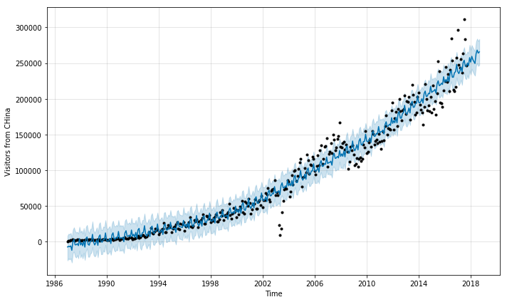
Prophet automatically detected monthly data and disabled weekly and daily seasonality. We can plot the forecast by Prophet
model_air.plot(forecast_air,xlabel='Time',
                             ylabel='Visitors from CHina')
Multiplicative Seasonality
We see that an additive model is not suitable; the predicted fluctuation due to seasonality is constant throughout the years. In reality we observe that the fluctuation is increasing. We can ask Prophet use multiplicative model instead by setting seasonality_mode='multiplicative'.
model_air=Prophet(seasonality_mode='multiplicative')
model_air.fit(air)
future_air=model_air.make_future_dataframe(periods=12, freq='M')
forecast_air=model_air.predict(future_air)
INFO:fbprophet.forecaster:Disabling weekly seasonality. Run prophet with weekly_seasonality=True to override this.
INFO:fbprophet.forecaster:Disabling daily seasonality. Run prophet with daily_seasonality=True to override this.
model_air.plot(forecast_air,xlabel='Time',
                             ylabel='Visitors from China')
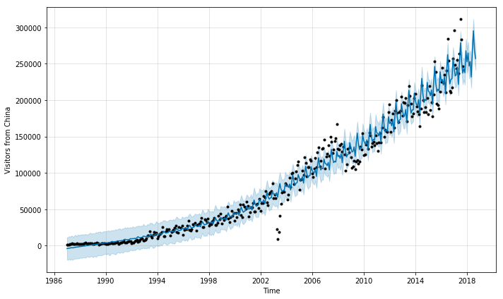
The seasonality effect increases over time with a multiplicative model.
Trend Change Points
The trend in a real time series can change abruptly. Prophet attempts to detect these changes automatically using a Laplacian or double exponential prior. By default, the change points are only fitted for the 1st 80% of the time series, allowing sufficient runway for the actual forecast. In the passenger arrival data, note that there is a sharp dip in 2003 due to the SARS outbreak in Singapore. These outliers should ideally be removed. Let’s display the change points detected by Prophet:
from fbprophet.plot import add_changepoints_to_plot
fig_air=model_air.plot(forecast_air)
a=add_changepoints_to_plot(fig_air.gca(),model_air,forecast_air)
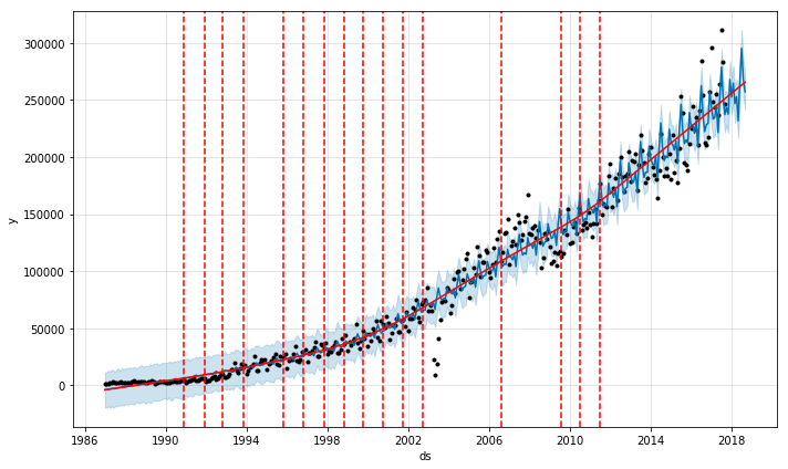
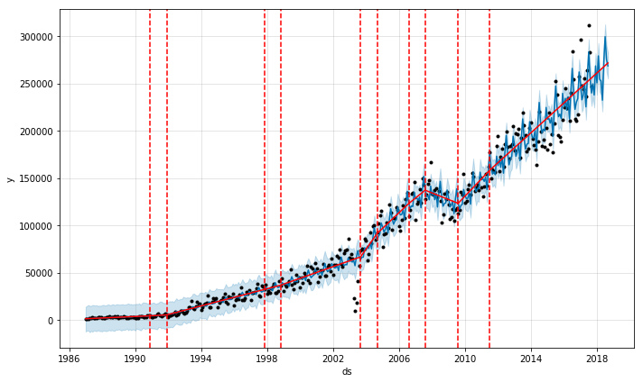
Visually it appears that the general trend is correct but it is being underfit. For example the decline during the 2008-2009 financial crisis is not detected. To adjust the trend change, we can use the parameter changepoint_prior_scale which is set to 0.05 by default. Increasing its value would make the trend more flexible and reduce underfitting, at the risk of overfitting. Let us set it to 0.5 as suggested by the Prophet Documentation Guide. If we want to generate uncertainty intervals for the trend and seasonality components, we need to perform full Bayesian sampling, which can be done by using the mcmc_samples parameter in Prophet.
model_air = Prophet(changepoint_prior_scale=0.5,
                    seasonality_mode='multiplicative'
                    )
forecast_air = model_air.fit(air).predict(future_air)
fig_air = model_air.plot(forecast_air)
a=add_changepoints_to_plot(fig_air.gca(),model_air,forecast_air)
INFO:fbprophet.forecaster:Disabling weekly seasonality. Run prophet with weekly_seasonality=True to override this.
INFO:fbprophet.forecaster:Disabling daily seasonality. Run prophet with daily_seasonality=True to override this.
Plot Model Components
We get a better fit of the trend when increasing changepoint_prior_scale. The decline during the financial crisis can be detected. The user can also manually define the change points based on domain knowledge (e.g. when forecasting sales the analyst might be aware of new product launches, sales, etc.) Using the plot_components function we can display the components of the model:
model_air.plot_components(forecast_air)
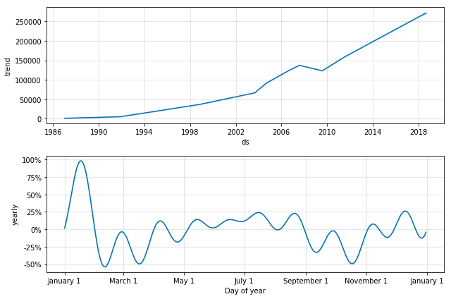
We observe a piecewise linear trend. Prophet also has the ability to fit saturating trends using a logistic growth trend model. This is applicable in cases where the trend is limited by capacity, e.g. the number of Facebook users in a country would be naturally limited by the number of people with access to the internet. This is done by setting the parameter growth=logistic and defining a column called cap in the dataframe.
Cross Validation
We can perform cross validation to measure forecast error. Cut off points are selected and we train the model with data up to that point. We can then compare the prediction vs actual data over a specified time horizon. This can be done using the cross_validation function. The parameter period specifies the interval between cut off points.
from fbprophet.diagnostics import cross_validation
df_cv = cross_validation(model_air, initial='4745 days',
                         period='365 days', horizon = '720 days')
INFO:fbprophet.diagnostics:Making 16 forecasts with cutoffs between 2000-09-15 00:00:00 and 2015-09-12 00:00:00
from fbprophet.diagnostics import performance_metrics
from fbprophet.plot import plot_cross_validation_metric

df_p = performance_metrics(df_cv)
df_p.head()
| horizon | mse | rmse | mae | mape | coverage | |
|---|---|---|---|---|---|---|
| 98 | 78 days | 2.480517e+08 | 15749.656257 | 11932.484783 | 0.094478 | 0.394737 |
| 146 | 78 days | 2.482712e+08 | 15756.623644 | 11972.847243 | 0.094157 | 0.421053 |
| 170 | 78 days | 2.479630e+08 | 15746.841395 | 11919.787650 | 0.093090 | 0.421053 |
| 266 | 79 days | 2.550821e+08 | 15971.290468 | 12338.291682 | 0.095245 | 0.394737 |
| 218 | 79 days | 2.547107e+08 | 15959.658037 | 12271.050843 | 0.093660 | 0.421053 |
Tanker Data - Additional Regressor
Let’s see how the Prophet performs on the oil tanker arrival data. We also explore the option of adding additional regressors. Additional regressors can be discrete like future holidays or another time series. However this time series needs to be know or forecasted separately for future dates .
In our example of tanker arrival data we limit the tanker arrival to the year 2016 and use the monthly oil price until 2018 from the World Bank as our additional regressor. The oil price is chosen as an example; in reality other parameters such as refining capacity, contango in the oil market, and storage levels might have more of an influence on the number of oil tankers visiting Singapore. Note that it is not always possible to predict these parameters in advance; this additional regressor can also be forecasted, with an associated forecast error.
tanker=pd.read_csv('D:/tanker-arrivals-breakdown-monthly.csv')

# Filter Data for Oil Tankers only
tanker=tanker[tanker.category == 'Oil Tankers']
tanker=tanker.drop(['category',
                    'gross_tonnage'],axis=1)

# rename columns
tanker = tanker.rename(columns = {'number_of_tankers': 'y',
                                  'month':'ds'})
# Load oil data
oil=pd.read_excel('D:/CMOHistoricalDataMonthly.xlsx',
                   sheet_name='Monthly Prices',
                   skiprows=6,
                   usecols=1
                   )
# Rename column and clean up date format
oil=oil.rename({'Unnamed: 0':'ds'},axis=1)
clean_oil = lambda x: x.replace('M','-')

oil['ds']=oil['ds'].map(clean_oil)
tanker=pd.merge(tanker,oil,left_on='ds',
                right_on='ds',
                how='left')
price=tanker['CRUDE_PETRO']
tanker=tanker[:180]
model_tanker = Prophet(changepoint_prior_scale=0.25)
model_tanker.add_regressor('CRUDE_PETRO')
model_tanker.fit(tanker)
future_tanker=model_tanker.make_future_dataframe(periods=20,
                                                 freq='M')
future_tanker=pd.concat([future_tanker,price],axis=1)
INFO:fbprophet.forecaster:Disabling weekly seasonality. Run prophet with weekly_seasonality=True to override this.
INFO:fbprophet.forecaster:Disabling daily seasonality. Run prophet with daily_seasonality=True to override this.
forecast_tanker=model_tanker.predict(future_tanker)
from fbprophet.plot import add_changepoints_to_plot
fig_tanker=model_tanker.plot(forecast_tanker)
a=add_changepoints_to_plot(fig_tanker.gca(),
                           model_tanker,
                           forecast_tanker)
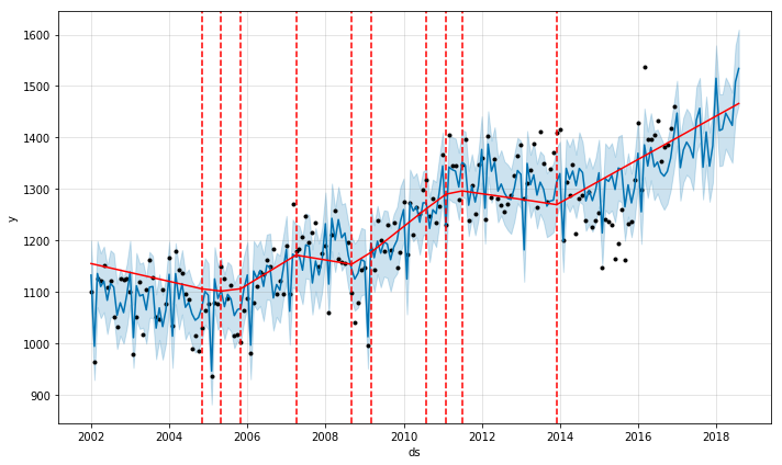
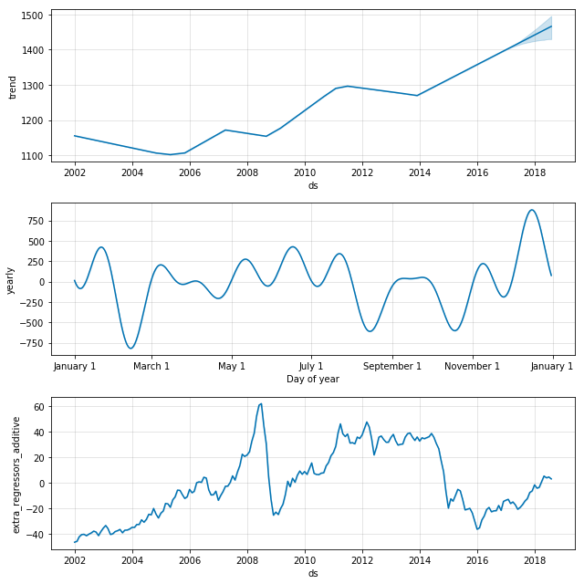
fig = model_tanker.plot_components(forecast_tanker)
Conclusion
Prophet is easy and intuitive to use and the components of the model are easily explainable. It also allows the incorporation of domain knowledge into the model, for example via known change points or capacity limits. The forecasts are pretty decent but in some cases certain parameters have to be tweaked compared to the default setting, which is easily done.